To copy data in alternate rows in Excel follow the step-by-step process given here. You can insert your required data in the alternate rows on selected columns.
How to Copy Data In Alternate Selected Rows In Excel (Step-by-step Process)?
There are a few simple steps that you have to follow to copy data to alternate cells given below.
Step 1: Copy and Paste Code to the Starting Cell
First of all, you have to copy the code =MOD(ROW(A1),2)=0 to the starting cell in Excel. When you paste the code to the cell, you will get a ‘FALSE’ text showing in the copied cell.
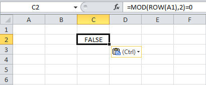
This is the code that creates an alternate different text when copied in the next step. It shows cell A1 inside the code when you check it. However, it does not mean that you only can copy it to column A. You can copy the code to any cell of your Excel sheet where you want to put data.
In the above example, the code is copied to column C and display ‘FALSE’ text.
Step 2: Copy This Cell to the End of the Required Cell
After you copy the code to the cell, you have to drag and copy the code to the end required cell. The end cell is the limit cell to which you want to put alternate data.
The copied code shows the alternate ‘TRUE’ and ‘FALSE’ text to alternate rows of a column. See the below image showing the content after you copy the code.
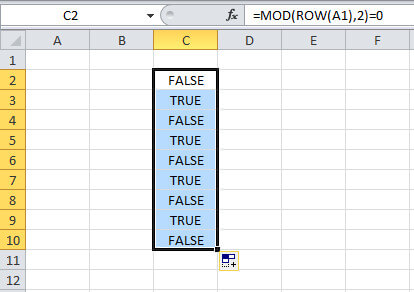
You can use the ‘TRUE’ alternate cell or ‘FALSE’ alternate cells as per your requirements. However, these steps use the ‘TRUE’ alternate rows to create alternate results easily in Excel.
Step 3: Go to the Start Cell and Click Filter Given Under Data>>Filter
Alternate text starts appearing where you have to add a filter option. To add a filter, you have to click the filter button given under the Data menu tab. This can be used to filter the required data from the given content.
The below image shows the place where you have to visit and click the filter option.
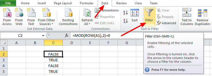
You can also use another method of selecting the filter option using only a keyboard shortcut. You have to visit the required place and press the keyboard button shortcut ‘ctrl’ + ‘shift’ + ‘L’. This will add a filter in the selected cell given in the above image.
Step 4: Click Filter Dropdown and Click only the ‘TRUE’ Checkbox in the Filter Dropdown
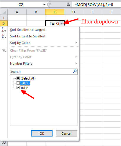
You have to click the filter dropdown given in the below image. The dropdown contains the various content options to select. In these options, you have to select only the ‘TRUE’ option and unselect other options.
Only the ‘TRUE’ text content starts to appear in the content. See the image below to check the content after selection.
However, you can also select the ‘FALSE’ option from the filter dropdown as per your requirement.
Step 5: Go to First TRUE and Enter Alternate Data to Copy
If you want to add the record to the ‘TRUE’ cells, you have to paste your required data in the first ‘TRUE’ text showing the cell. However, you can also use the ‘FALSE’ text cells to add data. This is the data content that you have to copy to the alternate selected rows.
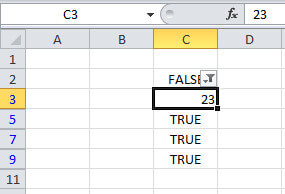
In the above example, we have chosen ‘TRUE’ cells to add the data. See the above image to add your data.
Step 6: Copy Paste the Same Data to Other TRUE Cells
You have pasted the data to the start cell. Now, copy the pasted data to all the ‘TRUE’ text cells. This adds the data to all the required cells. All you have to do is to remove the ‘FALSE’ showing cells in the next step.
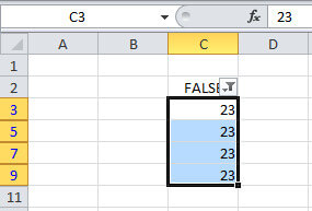
The above image shows the pasted data to all the required cells. You can change the data and copy and paste other data as per your requirements.
Step 7: Click Filter Dropdown and Click Only ‘FALSE’
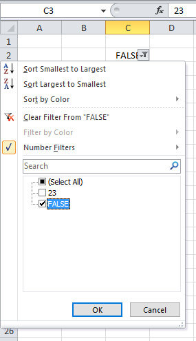
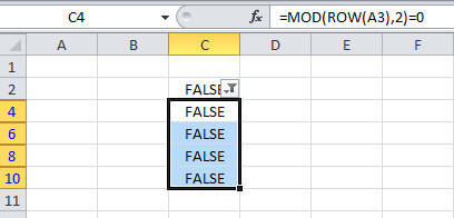
Now, you have to just remove the ‘FALSE’ cells and your alternate data is ready to display in Excel. To delete the ‘FALSE’ text cell, you have to first open the filter dropdown option. In the dropdown, select the checkbox for ‘FALSE’. This displays only the ‘FALSE’ cells as given in the image below.
Step 8: Last Step – Select and Delete All FALSE Cells
In the last step, you have to just select all the ‘FALSE’ cells and delete them. After the deletion, you will get only the required data in the required place in Excel.
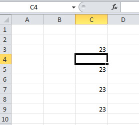
Final Output: Copy Data In Alternate Selected Rows
The below image showing the output contains the data in the alternate cells. You can add as many alternate data in the Excel sheet using this method.
You May Also Like to Read