In this tutorial, learn to use Cell Range In Excel with its different operations. A cell range is a collection of two or more cells to use in Excel formula. You can perform operations over single or multiple cells in MS Excel.
What is Cell Range in Excel
A cell range is a group of cells you select to use in functions and perform certain operations. The cell you have to use for the range is the intersection of rows and columns.
You can select multiple cells in a regular and irregular manner. To use the range in any function of Excel, you have to select the cell range with the method given below. You may also like to read post on rows and columns to create a cell in MS Excel.
Select Single Cell Range in Excel
A single cell is the intersection of the row and column of excel. If you click on any cell of the Excel sheet, you can find that it contains a column name and row name.
Let us take an example for the image given below. The below-selected cell is the intersection of column B and row 3. You can read the cell as the combination of row and column name as B3.
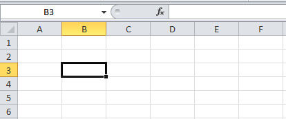
The same rule you have to follow the same naming rule when you select any cell.
Regular Multiple Range Selection
It the method of selecting multiple cells in a certain pattern like square, rectangular, etc. You can select the small and larger area of cells using this method.
To select your pattern, you have followed the steps given below.
Step 1: Go to start cell using mouse or keyboard.
Step 2: Hold ‘shift’ key of the keyboard.
Step 3: Click the last cell
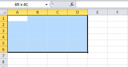
Example: Suppose you want to select the range (A1: D6) as you check in the above image. You have to first go to the cell A1 using your mouse or keyboard. Now, hold the keyboard ‘shift’ key and click the cell D6. This will select the required cell range as given in the above image.
Irregular Multiple Range Selection
An irregular selection is the selection of multiple cells without any patterns. You have to select any numbers of cells in Excel.
To select an irregular pattern, you have to follow the below-given steps:
Step 1: Click on the start cell using the mouse.
Step 2: Hold ‘ctrl’ key of your keyboard.
Step 3: Click the cells you want to select
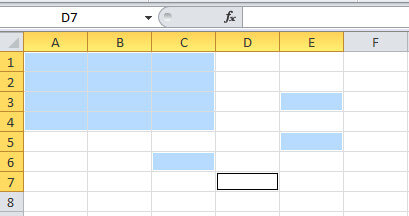
Example: Suppose you want to select the range (A1:C4,C6,E3,E5) given in the above image. Click the start cell or visit start cell using the arrow key of the keyboard. Now, hold the ‘ctrl’ key and click C4. Again click C6, E3, and E5 cells to select with the hold of the ‘ctrl’ keyboard key.
Column Range Selection Using Mouse and Keyboard
If you select all column cell, this also describes the range in Excel. To select all the cells of a column, you can use either your mouse or keyboard depend upon your choice. below are the methods to select all column cell.
Using Mouse
Step 1: Click the column cell name.
Using Keyboard
Step 1: Go the cell to select the column for.
Step 2: Hold ‘ctrl’ and press ‘space’ key of the keyboard.
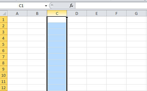
Example Suppose you want to select all the cells of column C given in the above image. You have to just click the column name C using the mouse.
If you want to select using the keyboard, you have to go the column C using arrow key. After that hold the ‘ctrl’ key and press the ‘space’ button of your keyboard. You may also like to read post on how to insert a new column in Excel using a keyboard.
Row Cell Range Selection with Mouse and Keyboard
To select all the cell range of a row, you can use a keyboard or mouse. For mouse use, you have to click the row name given to the left of the cell.
If you want to select all the row cell using only the keyboard, you have to follow the below-given steps.
Step 1: Go to the cell for the row you want using the arrow key.
Step 2: Hold the ‘shift’ key and press ‘space’ button of the keyboard to select the row.
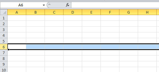
Example: If you want to select the row named 6 as given above. You have to click the name of the row using the mouse. You can also select a row using your keyboard shortcut. Go to any cell of row 6 using your keyboard arrow key. Now, hold the ‘shift’ key and push the ‘space’ bar of your keyboard.`
This will select the row with name 6. You may also like to read post on how to add a new row using MS Excel using the keyboard.
Get Range Selection for A Function of Excel
If you want to select the range from A1 to D7. Go to the cell A1 to start selecting the range. You have to select the range by pressing and holding the keyboard shift key. Now, click the cell D7 to complete the selection.
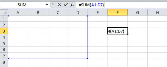
The range after selection showing in the function as SUM(A1:D7). See the image below showing the selection and the output of the sum function.
How to Autofill Numbers for the Selected Cell Range in Excel
Excel comes with many useful features to fill numbers in range. You can autofill range of number in multiple of 1, 2, 3, etc. You have to just grab the plus symbol creates when hovering over the cell. So, let’s create some useful autofill numbers in Excel.
Copy Same Number to Certain Cell Range
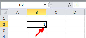
Step 1: Go to any cell( e.g.B2) and press the numeric 1 button.
Step 2: Mouse hovers over as indicated arrow location in the below image and holds the left mouse button. You will get a plus(+) sign in place of boxed mouse arrow sign.
Step 3: Drag the mouse to B7 to get the copy of the number 1 from cell B2 to B7.
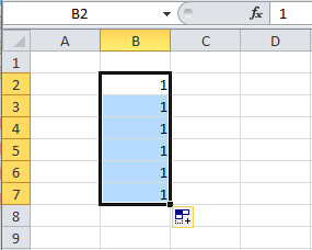
You can copy any number within a certain range using this method.
Autofill Number in Multiples of 2 to Certain Cell Range
Step 1: Go to cell B2, B3 and fill number by pressing button 2,4. In such a manner that 2 is in B2 and 4 is in B3.
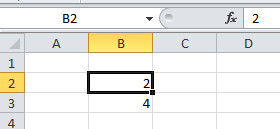
Step 2: Go to cell B2 and press and hold ‘shift’ key. Now, click the B3 cell while holding the ‘shift’ key. This selects the cell B2 and B3.
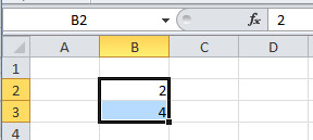
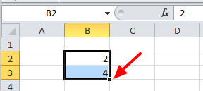
Step 3: Mouse hovers the indicated arrow location given below and holds the left button of the mouse. A plus(+) sign starts to appear in place of boxed mouse arrow sign.
Step 4: Now, you have to just drag the mouse to B8 to get the multiples of 2 from B2 to B8.
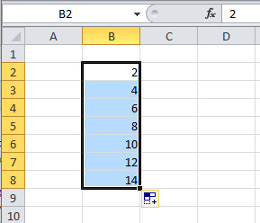
You can fill multiples of any number using the above method. All you have to do is to put the number in multiple first in step 1.
Autofill Dates in the Certain Cell Range in Excel
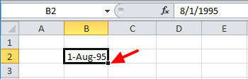
Step 1: Go to cell B2 and type 1-Aug-95.
Step 2: After typing date, hover over the indicated place given in the image and hold the mouse left button. plus(+) sign showing when you hover over the indicated place.
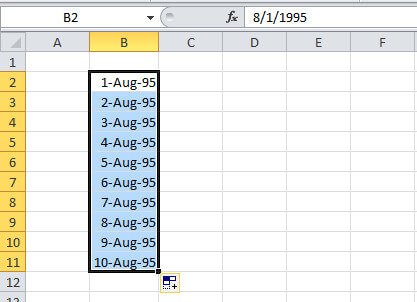
Step 3: Drag the mouse to B11 while holding the mouse left button. This will autofill the date range to a certain cell range.
Generate Sequence of Months in Cell Range in Excel
In addition to the above date format, you can also autofill the months. To perform this task and autofill months, follow the given below step-by-step method.
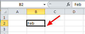
Step 1: Click the cell B2 and type Feb.
Step 2: Now, take your mouse to indicated place as given in the image and hold the mouse left button. A plus(+) sign displays when hovering over the indicated place.
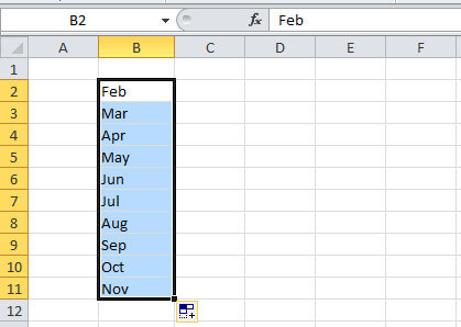
Step 3: You have to just drag the mouse down to the cell B11 with mouse left the button on hold. The selected cell range auto-filled with the sequence of months.
Hope, you like this post of cell range in excel with certain operations. If you have any query regarding the tutorial, please comment below.
Also tell me, what other operations you perform with the range in Excel